where N denotes the total sample size, μ ∗ the assumed treatment effect, σ 2 the variance of the observations, k the allocation ratio between treatment groups and qγ the γ-quantile of the standard normal distribution [2].
There have been various attempts to extend Formula (1) to multi-centre trials, e.g. by including a multiplicative factor to account for deviations from the standard design. Gallo as well as Ruvuna suggested such an inefficiency factor to account for centre size imbalances in the fixed effects setting [3, 4]. Both methods rely on the proportion of the treatment effects’ variances between balanced and imbalanced centre sizes, where the balanced case gives optimal power.
Van Breukelen and colleagues introduced an inefficiency factor for the mixed model [5]. This factor is based on the relative efficiency of unequal versus equal cluster sizes for the weighted least squares estimator, assuming a linear mixed effects model with an interaction between study site and treatment effect. Fedorov and Jones consider sample size formulas for balanced multi-centre designs and suggest simulations for more complex situations [6]. Vierron and Giradeau suggested a design-effect to adjust Eq. (1) for different study designs [7, 8].
All of the approaches mentioned above assume balanced treatment allocation by centre. Randomisation techniques such as block randomisation do not guarantee equal group sizes in all centres, especially if centres are small and block lengths are large. The normal approximation in (1) gives a lower boundary of the necessary sample size, but underpowered trials could occur, especially when between centre heterogeneity is large. We believe that this assumption is too strict for real trials and therefore suggest a sample size formula that accounts for unequal sample sizes.
It has been demonstrated that mixed models tend to yield better results compared to fixed effects models, especially when the number of patients per centre is small [9, 10]. For a small number of centres, however, the fixed effects design might result in better results, because the between-centre variation is likely to be estimated with bias in mixed models in that situation. We therefore aim to construct a sample size formula that accounts for baseline heterogeneity between study centres, assuming a linear mixed model for multi-centre designs.
Methods
Statistical model and estimators
We assume a linear mixed-effects model with a fixed intercept μ0, random effects uj, j=1,…,c to account for centre heterogeneity at baseline, and a fixed treatment effect μ. The data are assumed to follow some continuous distribution allowing for unequal sample sizes. The statistical model is given by
$$\beginfor pairwise independent uj, εijk with E(uj)=0, Var(uj)=τ 2 ∞, E(εijk)=0, Var(εijk)=σ 2 ∞, treatment indicator xi=1i=2> for treatment groups i=1,2, centres j=1,…,c and individuals k=1,…,nij for each treatment-centre combination. The shared random effect uj within centres induces the following covariance matrix \(Cov(Y_, \ldots, Y_>)=\bigoplus _^\left [\sigma ^\mathbf _>+\tau ^\mathbf _>\right ]\) , including all N observations with \(N=\sum _^\sum _^n_\) . Here, \(\mathbf _>\) denotes the nj-dimensional identity matrix and \(\mathbf _>\) the nj-dimensional matrix consisting of ones only with nj=n1j+n2j. We assume zero risk of contamination of the control group.
We are interested in differences between treatment groups and test the null hypothesis H0:μ=0 against the two-sided alternative HA:μ≠0. The distribution of the estimated treatment effect \(\widehat <\mu >\) can be approximated by a normal distribution, if the sample size is sufficiently large (say sample sizes larger 30). It follows
$$\beginThe null hypothesis can be rejected if the test statistic |T| exceeds the quantile q1−α/2 of the reference distribution for some fixed type I error rate α ∈ (0,1). In order to apply the statistical test, suitable estimators for the unknown parameters have to be chosen.
We choose \(\widehat <\mu >=\overline _-\overline _\) to measure treatment group differences, where \(\overline _=\frac >\sum _^\sum _^>Y_\) denotes the group mean in treatment group i. This estimator is unbiased, even if centres recruited patients for one treatment group only. The variance of \(>\) can be written as
Details on the derivation can be found elsewhere [8].
\(\text \left (\widehat <\mu >\right)\) depends on the overall sample size N, the variances σ 2 and τ 2 , and additionally the sample sizes by treatment group (N1, N2), number of study centres (c), and the sample sizes within study centres (n1j,n2j). In case of a perfectly balanced randomisation, the differences between centres cancel out and the treatment effect’s variance only depends on sample sizes N, N1, N2 and variance σ 2 , resulting in a sample size formula similar to (1).
The unknown variance parameters τ 2 and σ 2 can be estimated using the following quadratic forms
Additional assumptions for sample size calculation
Ni and nij are determined by recruitment and treatment allocation. We aim to replace all Ni, nij in (4) by their expectations that can be calculated based on the randomisation procedure and planned allocation proportion between treatment groups.
In the following, we want to calculate the overall sample size N and assume
- 1 a block randomisation stratified by centre with fixed block length b,
- 2 k:1 allocation ratio at each study site for k ∈ IN,
- 3 proportion of overall sample sizes between treatment groups according to allocation: N1=kN2.
Block randomisation
Since randomisation will not always result exactly in the planned allocation, we take a closer look at the randomisation process. Block randomisation with fixed block length b is a procedure where every b subjects get randomised between treatment groups at a time [11]. Complete blocks do always fulfil the planned k:1 allocation ratio. The block size should be unknown to investigators to strengthen the blinding in the trial.
In this article, we assume patients to be assigned to treatment groups i=1,2 within centres, for a fixed k:1 allocation ratio. This means that in each randomisation block b patients are randomized between treatment groups 1 and 2 in a way that for each patient receiving treatment 2, k patients will receive treatment 1. The set of randomisation tuples \(\Pi ^_\) depends on block length b and allocation parameter k. It is defined as follows
Treatment allocation imbalances can only occur in incomplete blocks with an upper boundary of kb/(k+1). The choice of k can be based on several assumptions as ethics, costs and other factors and will not be discussed further in this article. This topic is covered in more detail in a review by Dumville and colleagues [12]. It is available in many software packages and is therefore easy to apply [13, 14]. Further advantages and disadvantages of block randomisation are considered in the Discussion.
Derivation of the sample size formula
The underlying idea of sample size calculation is to find the overall sample size N, such that the quantile q1−α/2 of the reference distribution under the null hypothesis equals the quantile \(q^_\) of the reference distribution under a fixed alternative for type I and II error rates α and β.
Since we do assume a normally distributed test statistic, \(q^_\) can be approximated by a shifted N(0,1)-quantile \(q^_\approx q_+\frac <\mu >(\mu)>\) resulting in the following equation to construct a sample size formula
$$\beginBy isolating the sample size N, which is part of Var(μ), one can derive a sample size formula. In case of an ideal allocation, i. e., n1j=kn2j for all centres, (6) is equal to (1). Since this is unlikely to be observed, unbalanced designs are taken into account by incorporating expectations with respect to the randomisation procedure.
We derive the sample size formula for the general case of a k:1 allocation ratio and assume the overall treatment group sample sizes to fulfil N1=kN2 and therefore N=(k+1)N2. This leads to the set of randomisation tuples in (5). By taking assumptions 1-3, the variance of \(\widehat <\mu >\) given in (4) simplifies to
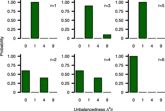
$$\beginwhere \(\Delta ^_\left (\frac >-n_\right)^\in \left [0, m^\right ]\) describe each centre’s imbalance that will result from incomplete blocks with m ∗ =b 2 /(k+1) 2 . The (discrete) probability distribution of \(\Delta _^\) depends on \(\Pi _^\) and the number of patients in the last block which equals the remainder of the Euclidean division rj=nj mod b. An example of \(\Delta _^|r_\) for a single centre is illustrated in Fig. 1.

The probability distribution of \(\Delta _^|r_\) is fully described by block length b, allocation parameter k and rj. For planning purposes it therefore seems reasonable to replace \(\Delta _^|r_\) by its expectation \(\text \left (\Delta _^|r_\right)\) to eliminate sample sizes n1j and n2j from (7). The expectation of the probability distribution can easily be derived as
$$\beginwhere p(·|rj) denotes the conditional density function of \(\Delta _^|r_\) . These expectations are shown in Fig. 2 for a single randomization block, k=1,2,3 and various block lengths b. Since the expected imbalance is the largest for k=1 we will restrict simulations to this case.

The expected imbalance between treatment groups \(\text \left (\Delta ^_|r_\right)\) increases with block length. This happens due to the fact that the probability to receive an incomplete randomisation block increases with increasing block length b. It is maximised when the last randomisation block only consists of \(\frac \) patients receiving treatment 1 or \(\frac \) patients receiving treatment 2, respectively. If we replace \(\Delta _^|r_\) by \(\text \left (\Delta _^|r_\right)\) , we can transform (6) into the following sample size formula for multi-centre trials (derivation is given in the appendix, see Additional file 1)
Simulations
General settings
We perform a simulation study to assess the accuracy of the sample size formulas in terms of statistical power using R, version 3.3.1 [15]. For each scenario, we repeat nsim=10,000 independent simulation runs. The R package blockrand is used for block randomisation [13]. All data are generated based on the statistical model described in (2), assuming a normal distribution for uj and εijk. The test statistic T given in (3) is used for all power simulations and it is approximated by a standard normal distribution under the null hypothesis. The effect of block randomisation is strongest for k=1, we therefore present simulation results for this setting only. The assumed effect size μ ∗ and values for variance components σ 2 and τ 2 are based on an example trial described in the next section. All code used for simulations is available in the Appendix, see Additional files 2, 3, 4, 5, 6, 7 and 8.
Subject-to-centre allocation
We consider equally as well as unequally sized study centres based on the following methods.
-
1 Equally sized study centres: Only in this situation, we can predict the sample size very precisely, since we can specify rj correctly prior to recruitment. Here, study centres are assumed to be equal. Since this assumption is limited to the fixed overall sample size N, we distribute the overall sample size to centres as follows
Example: The COMPETE II trial
Multi-centre trials are applied in many different disease areas. We present an example in the setting of disease management systems and use this trial to illustrate the sample size approach proposed.
Holbrook and colleagues conducted a randomized, multi-centre trial to investigate the benefit of an individualized electronic decision support system in adult patients diagnosed with type 2 diabetes [16]. This new intervention provided patient specific summaries and recommendations based on electronic medical records, aiming to improve the quality of diabetes management between patients and general practitioners. The tool was integrated into the practice work flow and offered web-based access by patients. In addition, an automated telephone reminder system was provided and all patients received a colour-coded printout quarterly. The control treatment consisted of usual care without use of this tool.
Primary outcome was a composite score difference compared to baseline. The composite score measured process quality on a scale from 0 to 10, based on the following parameters: blood pressure, cholesterol, glycated haemoglobin, foot check, kidney function, weight, physical activity, and smoking behaviour. The clinical targets are described in the original article. It was assessed at baseline and 6 months after randomization.
For this trial, 511 patients from 46 primary care providers were randomly assigned to intervention or control. At planning stage, the investigators aimed to recruit 508 patients to achieve 80% power to detect a difference of 1 for the primary outcome between treatment groups using a two-sided t-test with a type-1 error rate of α=0.05. No information on the assumed standard deviation is given in the article. Block-randomisation was stratified by study site in blocks of six, following a 1:1 allocation scheme.
The absolute measured improvement of composite scores between treatment groups was 1.26 (95% confidence interval (CI) 0.79-1.75; p-value < 0.001) favouring the new intervention.
Results
Approaches to sample size calculation
As long as no values for rj are assumed, Formula (9) cannot be used for sample size calculation. We consider a setting, where each centre will have at most one incomplete randomisation block. In the following, we present different ways to specify values of \(\text \left (\Delta _^|r_\right)\) for each centre prior to recruitment.
The resulting sample size formulas are listed in Table 1. More detailed explanations are provided in the following subsections.

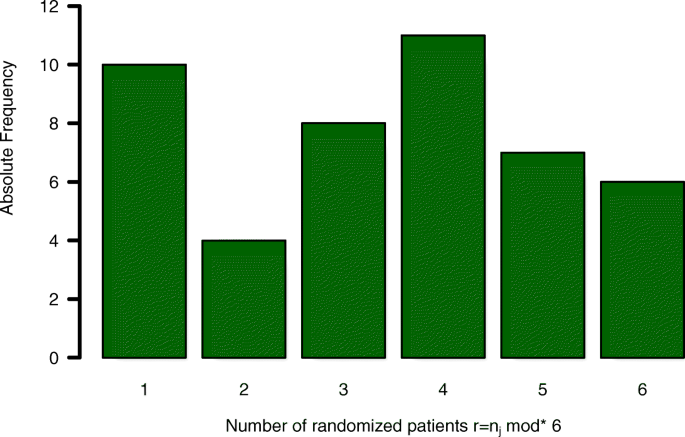
We use these numbers to illustrate the influence of unbalanced treatment group allocation on sample size and statistical power based on the assumed model. In total, 40 incomplete randomisation blocks (r<6) out of 46 study sites occurred. Based on the assumed model, statistical power of the analysis might be reduced due to those 40 incomplete randomisation blocks, compared to a trial, where the same amount of patients would have been recruited at a single centre.
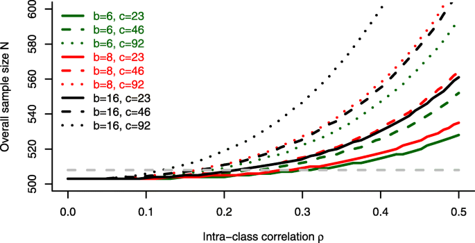
If we were to plan a new trial with similar features (μ=1, σ=4, type 1 and type 2 error rates α=0.05 and β=0.2, respectively) we could plug these values into the sample size formula \(N_<\mathrm

For a block length of b=6, as chosen in the trial, no substantial influence of the intraclass correlation ρ on the overall sample size can be observed. The reported value of ρ=0.08 in the trial would not require a sample size adjustment compared to the standard approach ( \(N^_>\) ). For larger block lengths, however, a strong increase of the estimated sample size can be seen, especially for ρ>0.2 and an increasing number of centres.
Power simulations
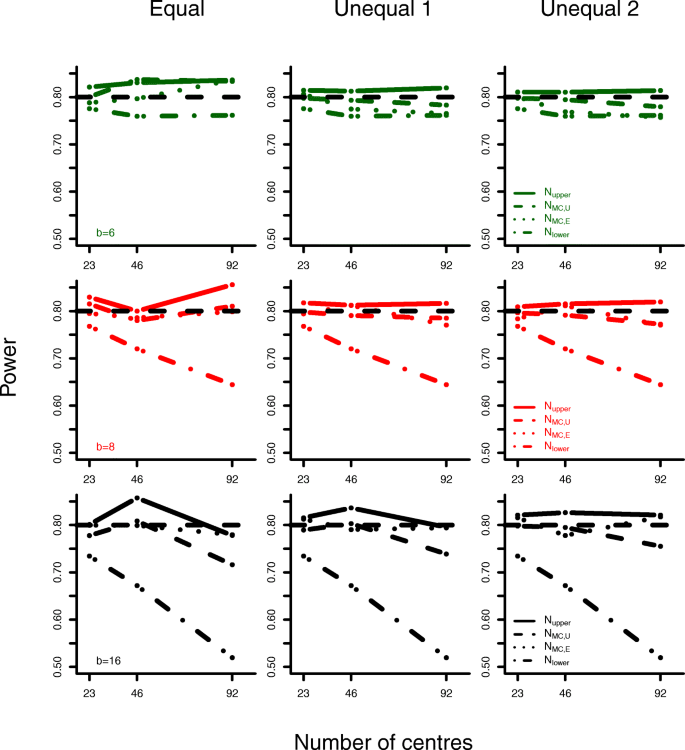
In addition to sample size calculations, we present some power simulation results for parameter settings based on the COMPETE II trial. We specify a treatment effect of μ=1, standard deviation σ=4 and intraclass-correlation coefficient ρ=0.5. Data was generated for various block lengths, numbers of centres and subject-to-centre allocation schemes. Resulting sample sizes and associated statistical power are given in Table 2 and Fig. 5.

Analyses based on the lower boundary formula do not achieve the planned power of 0.8. The deviance from the nominal level increases with block length and number of centres. The upper boundary formula results in power levels that exceed the nominal level slightly.
The new sample size formulas for equal and unequal centre sizes lead to reasonable power simulation results. Even if subject allocation is performed randomly in each simulation run (Unequal 2), adequate statistical power can be obtained.
Subject allocation might, by chance, result in more complete randomisation blocks for \(N_<\mathrm
Discussion
Patient enrolment and treatment allocation are key elements of every successful clinical trial. Randomisation techniques are used to achieve comparable treatment groups minimizing the risk of selection bias. Unfortunately, these randomisation procedures can result in unequal treatment group sizes and therefore a power loss compared to a balanced trial. Such imbalances cannot be determined prior to the trial, but we presented a way to estimate these values based on expectations.
The ICH E9 Guideline encourages the use of block randomisation and states the following on the choice of block sizes [1]: ”Care should be taken to choose block lengths that are sufficiently short to limit possible imbalance, but that are long enough to avoid predictability towards the end of the sequence in a block. Investigators and other relevant staff should generally be blind to the block length; the use of two or more block lengths, randomly selected for each block, can achieve the same purpose.”
The results shown remain valid when using variable block sizes, since incomplete blocks can occur using either method. Only the determination of expected values E(Δ 2 |r) is more complicated for variable blocks, because it depends on the range of block sizes used.
In a recent systematic review on prevalence and reporting of recruitment, randomisation and treatment errors in phase III randomized, controlled trials, stratified block randomisation was identified as randomisation technique of choice in 50% of 82 included studies published in New England Journal of Medicine, Lancet, Journal of the American Medical Association, Annals of Internal Medicine, or British Medical Journal between January and March 2015 [18]. The median number of participants per trial was 650 (range 40-84,496) and the number of centres varied between 1 and 1,161 with a median of 24. There are a number of trials that used fixed block lengths greater than 10 to allocate subjects between two treatment groups [19, 20]. Trials using random block randomisation almost never report the underlying block sizes, therefore we can not compare fixed versus random blocks any further. Overall, these observations support our idea to account for incomplete blocks to plan a multi-centre trial using either method for randomisation.
One limitation of our approach is a lack of knowledge on centre heterogeneity at the planning stage. There have been various articles with estimates of intraclass-correlation coefficients (ICC) derived from cluster-randomized trials. These estimates can be used to get an initial guess for centre heterogeneity in multi-centre trials. A nice overview is given in the following text book [21]. Also, the implementation of an adaptive sample size reestimation procedure could account for this problem as it has been applied for cluster randomized trials and the fixed effects multi-centre trial design [22–24]. The development of sample size reestimation strategies based on the approach proposed here is subject to ongoing research. When planning an individually-randomized multi-centre trial there is a risk of control group contamination. This can partly be handled in placebo-controlled pharmacological trials or when proper blinding of patients and researchers is implemented [25]. Alternatively a cluster-randomized trial could be used to prevent contamination of treatment groups. This would, however, be associated with a higher sample size compared to the multi-centre design [26].
Here, we assumed a constant treatment effect across the centres. This is in line with the ICH E9 Guideline, which demands to avoid treatment-by-centre interactions in the primary analysis [1]. Therefore, this is at least for the planning of a trial an adequate assumption. Nevertheless, sensitivity analyses might explore treatment-by-centre interactions. Extending the sample size approach to a model including treatment-by-centre interactions is subject to future research.
Conclusion
Imbalances in treatment allocation will lead to a power loss in multi-centre trials, if baseline heterogeneity is present. This risk can be accounted for when using appropriate methods for sample size calculation. To reduce uncertainty of sample size calculation, we recommend to calculate lower and upper boundaries in addition to the sample size.